The Algorithm

Breadth first traversal (usually interchanged with breadth first search), is a graph traversal algorithm that works in a level order manner. Our graph is defined as G={V,E}, where V is a set of vertices and E is a set of edges.

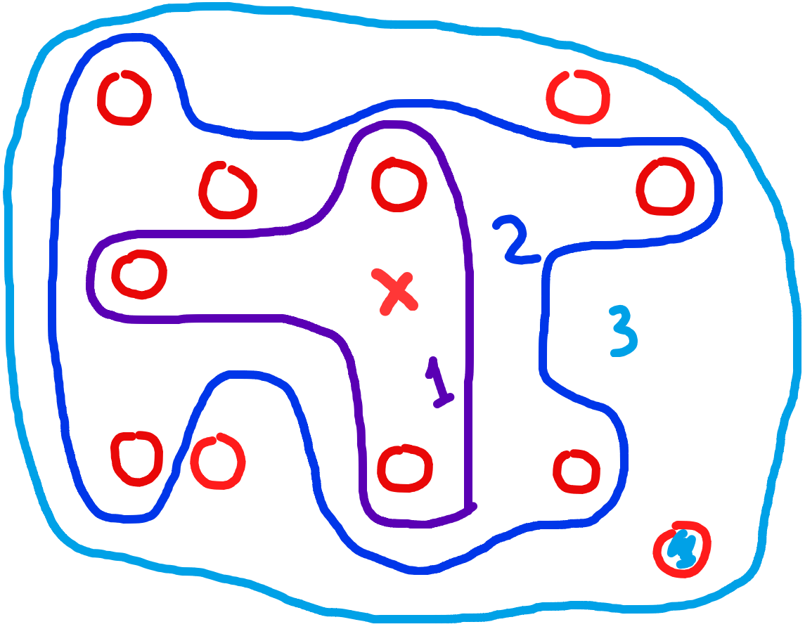
In more intuitive words: you start from some point on a graph and expand outward one level at a time. The first level is simply one node, and the next levels are simply all the nodes near a node in the previous level (see the colorful graph on the cover of this post).

The algorithm also doubles down as a single source shortest path (SSSP) algorithm on unweighted graphs.

Below is the pseudo-code for breadth first search. I’ve coded it so that you can -instead of modify the funciton to make it do what you want- fill in the callback function named on_visit.

input: adjacency list
output: shortest path tree

function bft(G, on_visit):

    q = [0]

    while q not empty:

        node = q.popLeft()
        on_visit(node)
        mark current as visted

        for neighbor in G[node]:
            if neighbor not visted:
                q.addRight(neighbor)

Key Points:
level-order traversal
implicitly traveses shortest path tree on an unweighted graph
can pass in a callback to execute upon visiting a node

Analysis

Runtime for an Adjacency List

The runtime of breadth first traversal depends on the type of graph provided as input. In the snippet above I’ve implied that the graph is an adjacency list. Why? If you look at the for loop, you’ll notice that G[node] is a collection of neighbors of node.

G = [
    [...],
    [...],
    [...]
]

So in an adjacency list, if we wanna find all neighbors of a vertex v, we get access to the neighbor collection in constant time (O(1)), which again we access through G[v]. That said, the following is the algorithm runtime:

visting all vertices: O(V)
visiting all neighbors of all vertices: O(E); for each vertex v this costs O(#neighbors(v)), which by definition sums to O(E)
total:
    O(V) + O(E)
    = O(V+E)

Runtime for an Adjacency Matrix

The alternative to an adjacency list is an adjacency matrix. Think the Pokémon type chart, where if two vertices (types in this case) are related, the cell they intersect at captures the relationship. Below is a simplified version of the type advantage chart.

G[row_type][column_type] == 1 means the row type beats the column type.

G = [
    #FIRE   WATER,  GRASS
    [0,     0,      1],   #FIRE
    [1,     0,      0],   #WATER
    [0,     1,      0]    #GRASS
]

If we wanna find all the vertices related to a given v in an adjacency matrix, we can’t just use G[v]. We need to also filter by the edges that equal 1, which costs O(V) per vertex we visit. Given all this, below is the analysis:

visting all vertices: O(V)
cost per visit: O(V); again must filter through all vertices to find neighbors
total: O(V^2)

TL;DR

The bottleneck for the runtime of breadth first traversal is the neighbor-finding part of the algorithm. In an adjacency list that step costs O(1), and in an adjacency matrix that step costs O(V).

Runtimes:
BFT on adjacency list: O(V + E)
BFT on adjacency matrix: O(V^2)

The way I learned algorithms [Ad]

Note

Please excuse the wordiness of this post - I lost the drawings that I would’ve used for this post, so I decided to keep it wordy and post my relevant YouTube short here, as well as the code and the key points.

Subscribe to the channel if you haven’t already!

The Algorithm#

Analysis#

Runtime for an Adjacency List#

Runtime for an Adjacency Matrix#

TL;DR#

Note#